
Generative models are a type of machine learning model that are designed to generate new, synthetic data samples that are similar to a training dataset. In the context of reservoir engineering, generative models could potentially be used to generate synthetic reservoir models for use in simulation and analysis.
There are a number of different approaches to using generative models for reservoir engineering. One approach is to use a generative model to synthesize a large number of different reservoir models, and then use these synthetic models to perform uncertainty analysis or sensitivity analysis. This could help engineers to better understand the range of possible outcomes for a given reservoir, and to identify key factors that might impact production.
Overall, the use of generative models in reservoir engineering is an active area of research, and in this article we are going to take a closer look on using GANs to incorporate uncertainty on the geostatistical workflow.
The old way
First, we need to introduce some concepts - like Training Image (TI) and the SNESIM algorithm. In the context of geostatistical analysis, the TI is a representation of the spatial distribution of a given property or variable of interest within a reservoir. It is typically derived from a combination of data sources, including well logs, core samples, and geophysical surveys. The training image is uncertain as the ground truth spatial pattern is unknown. For example, the expert geologist may know that a meandering river constitutes the depositional setting of an oil reservoir. However, the river width and sinuosity of the river are still unknown.
As for the algorithm used - the Single Normal Equation Simulation (SNESIM) has been widely used in the geostatistical literature. The algorithm follows the sequential paradigm, that is, the simulated value act as a data value to simulate the next node. The SNESIM algorithm may be summarized in the following steps:
- Migrate the conditioning data to the simulation grid;
- Scan the training image with a template and build a search tree that contains the probabilities associated with all possible data events;
- Define a random path that visits all the nodes in the simulation grid;
For each node u in the simulation grid, do:
- Search the nearby data and define the corresponding data event;
- Get the probabilities associated with the data event from the search tree and build the conditional probability density function (cpdf);
Draw a simulated value for node u from the cpdf and add it to the dataset.
- Steps 3-4 are repeated to generate another realization.
The major drawback of the SNESIM is its high RAM usage. Despite this limitation, the SNESIM has been successfully applied to numerous case studies. The case studies include simulations of oil reservoirs and mineral deposits.
The traditional workflow is best summarized in the figure below. This workflow starts with a TI provided by the expert geologist and the hard data. Once we have all the data necessary for the simulation, we can run the realizations using the SNESIM algorithm.
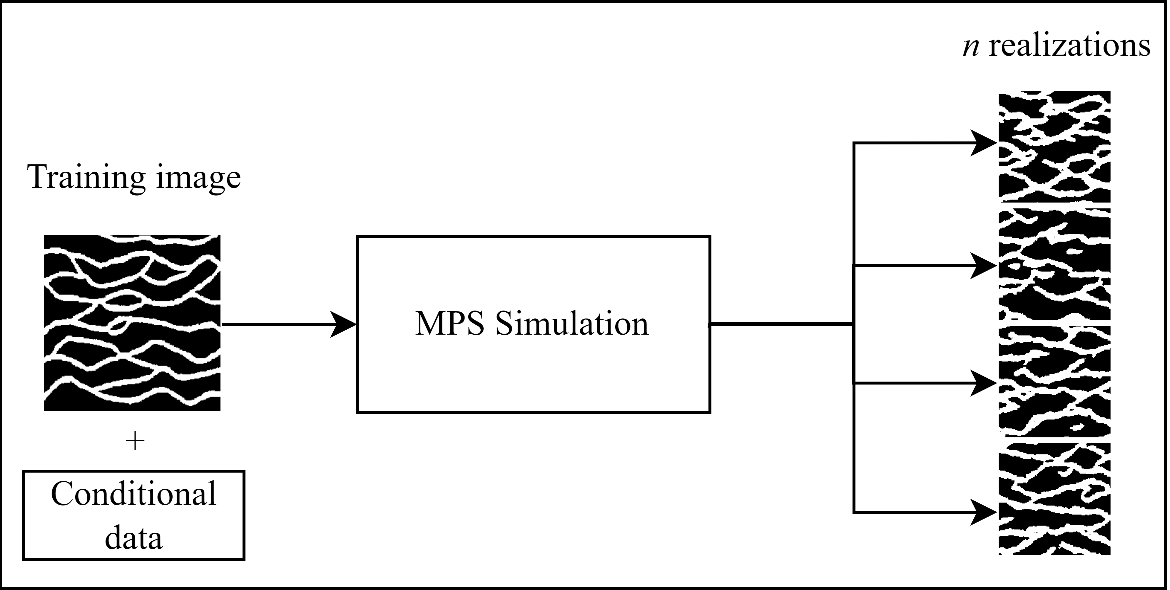 Traditional workflow diagram.
Proposed workflow
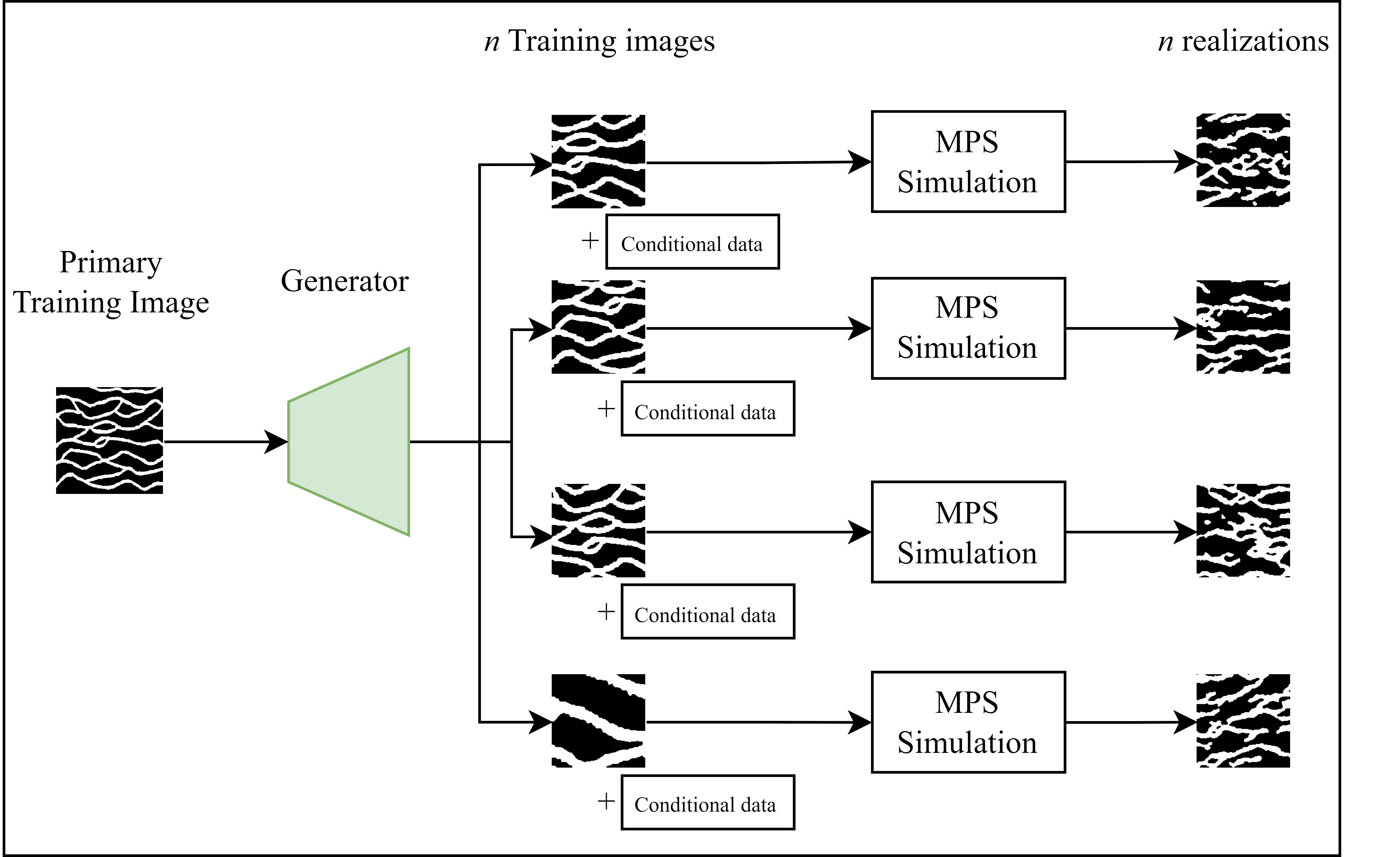
We suggest using Generative Adversarial Networks (GANs) to add TI uncertainty into the MPS geostatistical approach in this method. The addition of the TI uncertainty involves the creation of many TIs before running the MPS simulation (see figure below). Since the sliding windows dataset from the TI is already part of our database, we need the generative network to learn the implicit distribution of the dataset through the training process of this neural network.
The Generator learns how the distribution of a TI similar to primary TI is and, according to its classification, whether real or fake, the models have their weights updated. This process is iterative and results in the Generative Neural Network model. The model can build TIs whose distributions are similar to those of the primary TI. Only after these preliminary steps we can start to use the model as a TI Generator. Given this, the other part of the workflow can be summarized in the following steps:
- Build a dataset of Training Images using Generative Adversarial Networks;
- Select appropriate TIs created;
- Build simulated models using MPS simulation using the TIs selected;
- Check the results.
The SNESIM parameters for this workflow are the same as those used in the traditional workflow.The only difference is that the traditional workflow uses one TI for all realizations, while the proposed workflow uses one TI for each realization. The GAN generated all TIs used in the proposed workflow.
 Proposed workflow diagram.
Results
Figures above show four randomly built realizations with the traditional and proposed workflow. The results show that both workflows reproduced the curvilinear features from the original Training Image. The simulation results in the proposed workflow also reproduced the desired features with similar channel width.
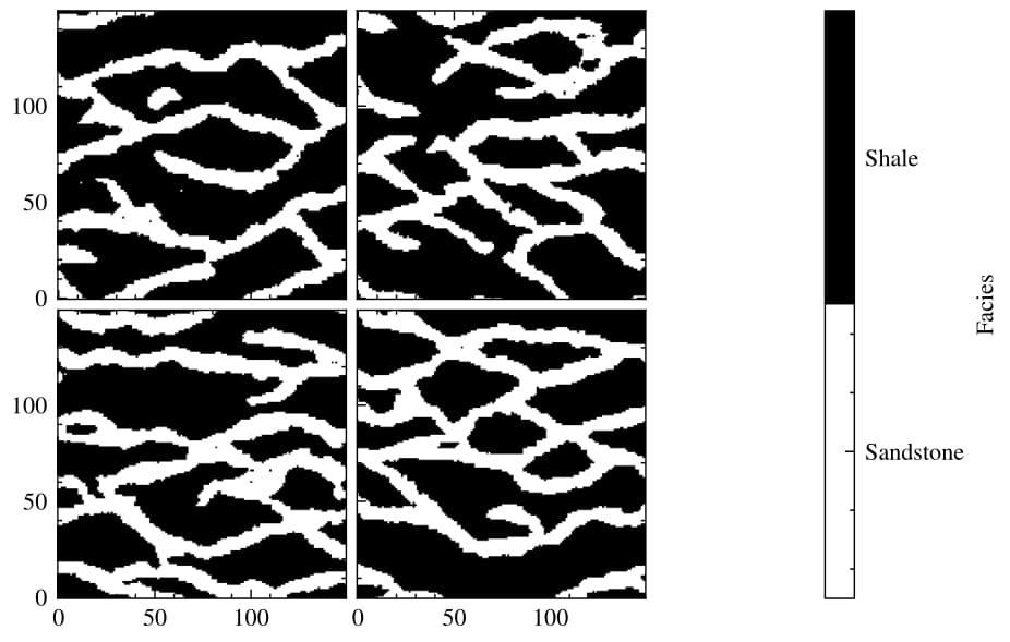 The image grid contains four realizations from the traditional workflow.
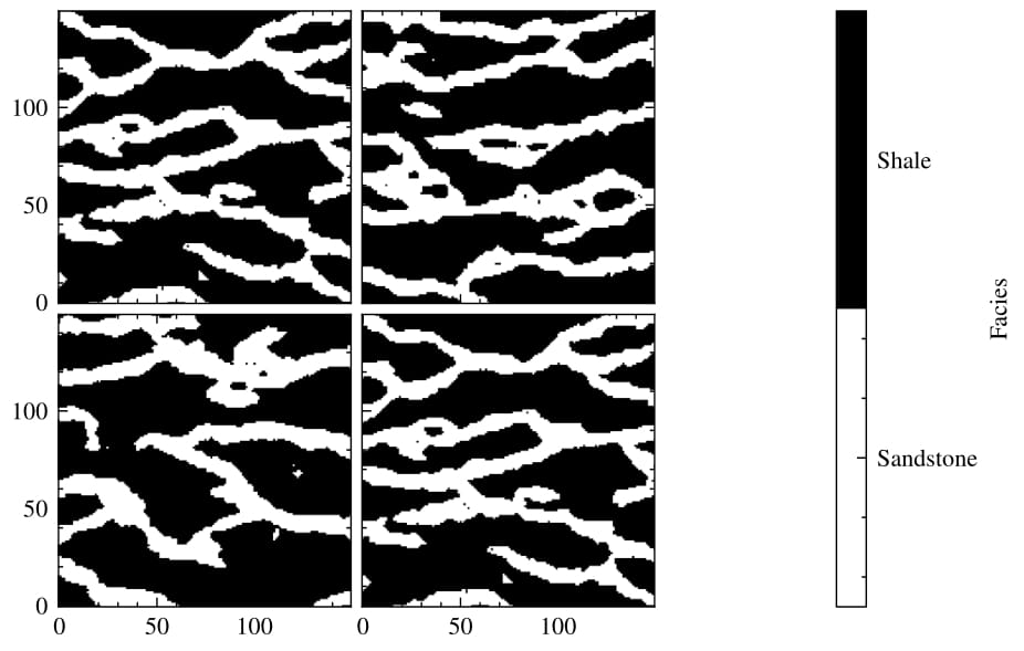 The image grid contains four realizations from the proposed workflow.
The next plot compares the facies proportions between the primary Training Image and the simulated models for all realizations built using the traditional and proposed workflows. As expected, the simulations reproduced the global facies proportions, confirming that the generative model can learn the proportions from the dataset. The results show that the simulated models do not have global bias. We can also see that the simulations from the proposed workflow can produce more images with shale.
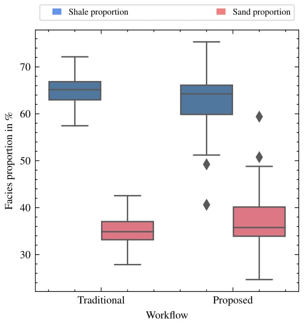 The boxplots displaying the facies proportion for each workflow.
From the 100 models generated for each workflow, E-type maps of the spatial distribution of the facies were generated by calculating the point average of all realizations. The E-type shows the probability of being a certain category for all grid nodes. For instance, consider a grid node where 90 realizations are sand and 10 realizations are shale. At this location, the probability of being sand (E-type of sand) is 90%, while the probability of being shale (E-type of shale) is 10%. The figure below shows the E-type for the traditional and proposed workflows for sand. The E-type for shale is one minus the E-type estimate for sand and was omitted to make the paper more concise. Note that, the traditional model has well defined contours and channels, while for the proposed workflow, the blurred area implies higher uncertainty of the model.
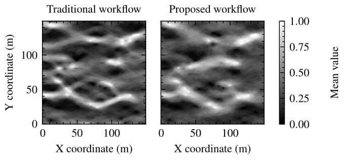 E-type estimate for sand of each workflow.
A multidimensional scaling representation using Euclidean distance of the simulated models can be observed in the next plot. To ensure that the Euclidean distance between any two points reproduces the dissimilarity in the matrix, a 3D mapping space is considered fit. Note that the simulated models obtained with the proposed workflow are more scattered compared with those obtained with the traditional workflow. This result demonstrates that the proposed workflow represents better the space of uncertainty.
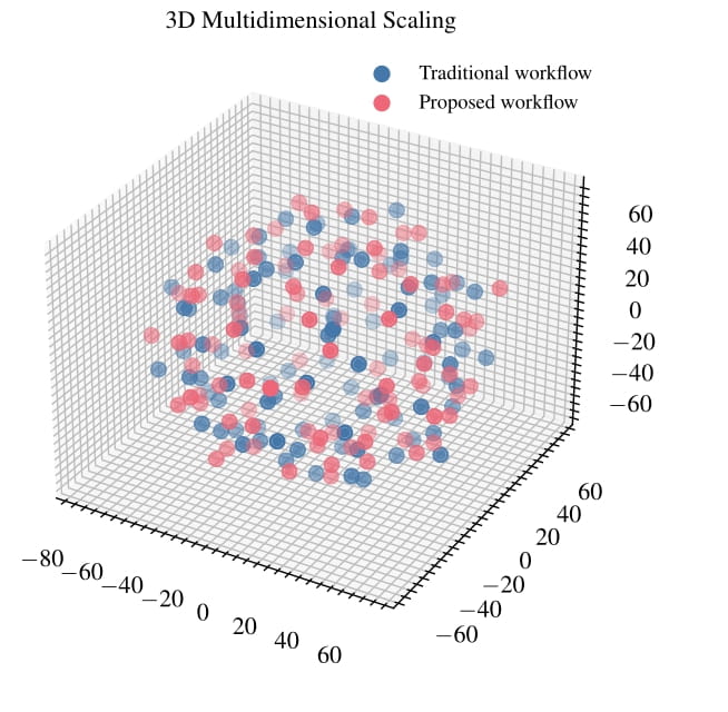 The multidimensional scaling analysis represented in a 3D space.
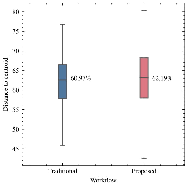 The boxplot with distances from each point to workflow centroid, the boxplot shows the median value for both workflows.
Also, the boxplot of the distances between the simulated models and their cluster centroids confirms the observation made. We can see that the average distance between models is 1.99% higher for the proposed workflow.
Final Remarks
The adversity with employing MPS geostatistical methods is that the uncertainty associated with the TI is ignored. We proposed the use of GANs to add uncertainty into the TI, such that each realization depicts a conceivable geological situation.
The study shows the capacity of GANs to generate realistic training images. Moreover, the proposed workflow, which combines GAN and SNESIM, resulted in a better exploration of the space of uncertainty. The spread of the global facies proportions and the local uncertainty is higher for the proposed workflow. This result was also visible in the MDS representation of the simulated models. The simulated models using the proposed workflow were more scattered in the MDS space. The increased variability of the simulated models improves the decision-making process, as the decisions must deal with very different scenarios.
Simulated models that are too similar underestimate the possible outcomes that may occur when the reservoir is exploited.