
While digging through some articles and theories in geostatistics, there are a set of concepts that are really important to understand. Below, we have some engineering-type definitions to these concepts.
The random variable concept
Random variable (RV), well what can I say more? It is almost self-explainable :D. Let us consider $Z$, a variable that can be either a discrete, or continuous. In the first case, the $n$ occurrences of the $Z$ variable can only assume a finite amount of values, an example of a categorical variable can be seen as lithology or facies value which are restricted to categories such as “Sandstone”, “Greenschist”, and so on…The probability of occurrences must follow the condition $\sum_{i=1}^{N}p_i = 1$, that is, all categories probabilities must sum up to 1.
As for the continuous variable, it can assume ANY given value within an interval. Given a porosity value, the random variable is continuous from 0-100% and its cumulative distribution function (cdf).
\[F(z) = Prob(Z \leq z) \in 0, 1\]Similarly, intervals can be calculated with
\[Prob(Z \in (a,b]) = F(b) - F(a)\]A nice way to weighted average - mathematical expectation
Mathematical expectation is like an average of a bunch of numbers. Formally speaking, the mathematical expectation of a discrete random variable $Z$ is defined as the sum of the product of each possible outcome of $Z$ and its corresponding probability, given by:
\[E(Z) = \sum z_i * p(Z=z_o)\]Where $z_i$ are the possible outcomes of $Z$ and $p(Z=Z_i)$ is the probability of $Z$ being equal to $z_i$.
For a continuous random variable $Z$, the mathematical expectation is defined as the integral of the product of $Z$ and its probability density function (pdf) over its range:
\[E(Z) = \int z*F(z) dz\]Where $F(z)$ is the pdf of $Z$.
In geostatistics, the expectation plays a crucial role in understanding the underlying patterns in spatial data. The expectation provides a measure of the central tendency or average behavior of a random variable, which can be used to make inferences about the population from which the data was collected.
For example, if we have a set of spatial data representing the average annual rainfall in different regions, the expectation of the rainfall can be calculated and used to understand the average rainfall across all regions. This information can then be used to make decisions regarding water management, agriculture, and other industries that rely on rainfall.
In addition, the expectation can also be used to model the spatial dependencies between different regions. For example, if we observe that two regions have similar rainfall patterns, we can assume that there is a spatial dependence between them and model it using spatial regression techniques.
Overall, the expectation is a useful tool in geostatistics for characterizing the central tendency and dependencies in spatial data, and for making informed decisions based on these patterns.
Linear property of the expected value
The expected value has a linear property, which states that the expected valu of a linear combination of random variables is equal to the linear combination of their expected values. This property can be clearly written as below, considering $Z$ and $Y$ RVs and $a$, $b$ as constants:
\[E(aZ + bY) = aE(Z) + bE(Y)\]This property is extremely useful, as it allows us to find the expected valu of a complex function by finding the expected value of each component and combining them linearly.
What Gauss has to do with it?
In case you never heard about the Gaussian or Normal Distribution - the Gaussian model is like a magic that can help us understand how things are spread out. The Gaussian model says that our variables are spread out in a special way, like a bell shape. The middle of the bell is the mean ($\mu$) value, and the numbers get less and less common as you go to the sides of the bell.
The Gaussian model is also both defined by its $\mu$ and standard deviation ($\sigma$). The pdf of a Gaussian distribution is given by:
\[Z \sim \mathcal{N}(\mu,\,\sigma^{2})\] \[\mathcal{G}(z) = \frac{1}{\sigma\sqrt{2\pi}} e^{-\frac{1}{2}(\frac{z-\mu}{\sigma})^2}\]Where $z$ is a RV representing the normal distribution.
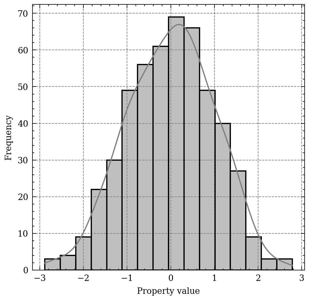 The bell-shape of the normal distribution.
Lognormal model
The lognormal distribution is a continuous probability distribution that is defined by the exponential of a normally distributed random variable. The distribution can be written as:
\(Z_{lognormal} = e^{Z}\).
Considering $Z$ a normally distributed curve with mean $\mu$ and standard deviation $\sigma$. The lognormal distribution is characterized by (a) its mean and variance ($\mu, \sigma^2$); (b) or its mean and variance ($\alpha, \beta^2$) of the log transform $Z_{lognormal} = ln(Z)$
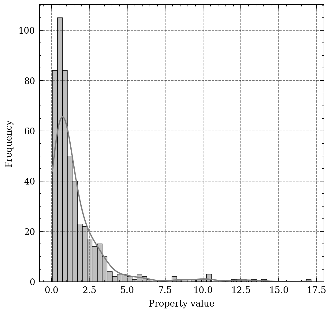 The shape of the lognormal distribution.
Even though the Gaussian model is very convenient, the log-normal distribution has several advantages over the Gaussian distribution in certain applications - as most earth science variables are non-negative valued and its distributions tend to be skewed, this modelling seems more fit.
Bivariate distribution
Given the two modelling approaches, they are only for one variable at a time, be it $Z$ or the sum $Y = \sum_{i=1}^{n}Z_i$ of $n$’s variables. And a little bird once told me that, in geostatistics, it is kind of important to know the pattern of dependence from one $Z$ variable to another $Y$.
A bivariate distribution refers to the relationship between two variables in a dataset, where each variable has its own set of values and the distribution represents the joint probability of these values occurring together. For example, in a study of the relationship between rainfall and soil erosion, the bivariate distribution would show the frequency with which different levels of rainfall are associated with different levels of soil erosion. This type of analysis helps in understanding the interdependence of variables and can be useful in making predictions or understanding cause-and-effect relationships in earth science phenomena.
\[F_{ZY}(z, y) = Prob(Z\leq z, Y\leq y)\]The bivariate equivalent of a histogram is scatterplot, where each pair is plotted as point, see the figure below.
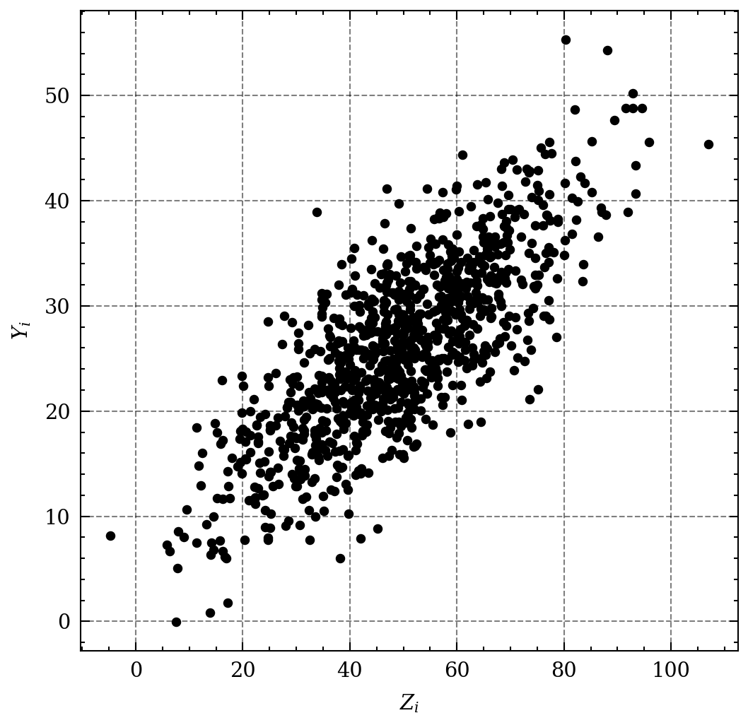 The pair $Z, Y$ scatter.
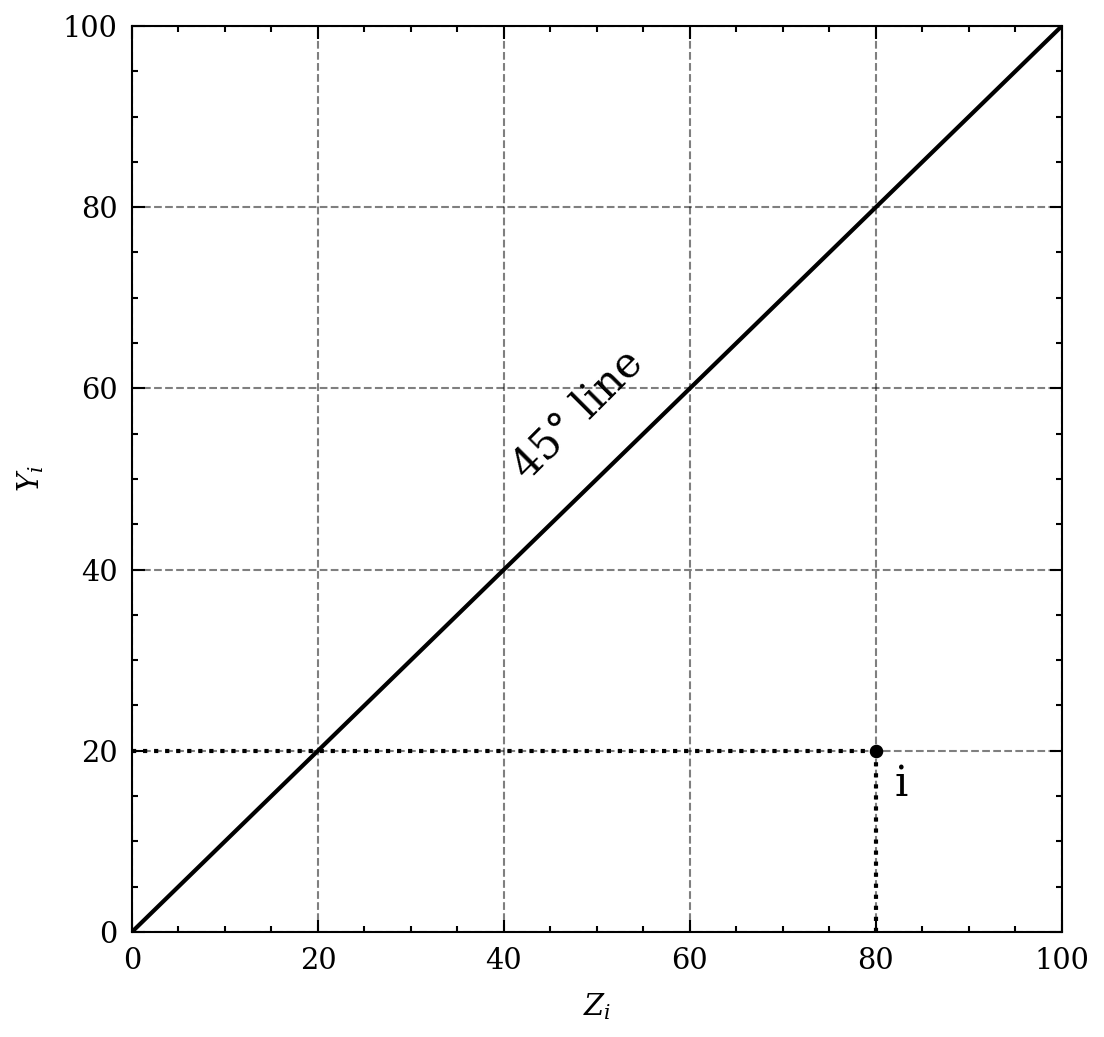 A scatterplot of a single sample, comparing to XY line.
The expected value of the product ZY as the bivariate probability-weighted average of the join outcomes ZY=zy;
\[E(ZY) = \int\int_{-\infty}^{\infty} z y f(z, y) dzdy\]Where, $f_{ZY}(z, y) = \frac{d^2 F_{ZY}(z, y)}{dz dy}$ is the bivariate probability density function. The bivariate moment is a statistical concept that refers to the measurement of the relationship between two variables in a bivariate data set. It is calculated as the expected value of the product of the two variables and is a measure of their association or correlation. The first bivariate moment is the covariance and the second bivariate moment is the correlation coefficient. These measures can provide insight into the strength and direction of the relationship between the two variables and are commonly used in statistical analysis.
The covariance is defined as:
\[Cov(Z, Y) = E(ZY) - \mu_Z * \mu_Y\]It is worth mentioning that although the variances $\sigma_Z^2$ and $\sigma_Y^2$ are necessarily non-negative, the cross-covariance $\sigma_{ZY}$ may be negative if there a positive or negative deviation. Ergo, the coeficient of correlation $\rho_{ZY}$ between the two random variables $Z$ and $Y$ is a covariance standardized to be unit-free.
\[\rho_{ZY} = \frac{\sigma_{ZY}}{\sigma_{Z} \sigma_{Y}} \in [-1, 1]\]In summary, covariance measures the linear association between two variables, indicating the extent to which two variables change together. It gives an idea of the direction of the relationship, but not the strength. Correlation, on the other hand, is a normalized version of covariance that measures the strength of the linear relationship between two variables. It provides a value between -1 and 1, with -1 indicating a strong negative correlation, 0 indicating no correlation, and 1 indicating a strong positive correlation.
Final Remarks
In this lesson, I hope you could review or learn more about core concepts in geostatistics. In conclusion, statistics and earth sciences are two fields that are highly interrelated and complementary. Understanding the concepts of statistics is crucial in earth sciences, as it helps to analyze, interpret and make sense of complex data generated from various sources. On the other hand, earth sciences provide rich data that can be used to test and refine statistical models.
The integration of these two fields helps to address complex environmental and geological questions, and provides valuable insights into the functioning of our geological structures. With continued advances in both areas, it is likely that the relationship between statistics and earth sciences will only grow stronger and more essential in the years to come.